• What is ClimateSimTM?
• Target audience
• How to use ClimateSim
• Climate model in ClimateSim 1.0
• What is next for ClimateSim?
• References
ClimateSim is a fast and simple climate modeling and simulation tool. It is a web app that is freely available to all students, teachers, policymakers, journalists and others interested in climate science. ClimateSim allows users to model scenarios of greenhouse gas (GHG) emissions in the current century and simulates the first-order response of the earth system.
ClimateSim is based on an emissions-driven, coupled climate-GHG cycle model. It converts a user-selected or user-defined emissions scenario into atmospheric concentrations of greenhouse gases over time, and then computes the earth system’s response – including the global mean surface temperature change/anomaly over time as well as latitudinal mean surface temperatures.
In addition to the temperature response, ClimateSim reports a number of other critical climate variables (such as radiative forcing, radiant flux densities, atmospheric longwave emissivity, and albedos) to help users connect the simulation output to theory and models.
ClimateSim models details such as the land/ocean carbon uptake (including climate-carbon feedback), lifetimes of non-CO2 GHGs, ice-albedo feedback, and equator-to-pole heat transport. The current 1.0 version uses an extended one-layer atmospheric model (to be expanded to a multilayer model in 2.0).
Note that ClimateSim is not based on a general circulation model and is not designed to be used for rigorous predictions of future climate – it is an educational tool for teaching and learning introductory climate science.
ClimateSim is listed in the National Science Digital Library, MERLOT, EdSurge and LearnPlatform databases as an online science education tool, and is also available through the
LibreTexts open-access textbook project.
The current version of ClimateSim is 1.0.
ClimateSim is targeted to undergraduate and advanced high-school students in physics, geoscience, and environmental science courses. We developed ClimateSim to be a science education tool primarily that can be used as a virtual lab. It makes climate simulation accessible in a simplified form to all students and provides an easy-to-use simulation platform for performing virtual climate experiments. Instructors can use ClimateSim to illustrate climate-change concepts, demonstrate dynamic relationships between climate variables, and assign simulation-based exercises as part of their courses.
ClimateSim is also an appropriate and accessible tool that policymakers, journalists and others can use to get a better understanding and working knowledge of the basics of climate science.
1. Use the Select Scenario dropdown menu to select an emissions scenario. Available scenarios include the four key IPCC scenarios and other representative GHG emissions scenarios. All scenarios run from the year 2011 through 2100. Each scenario includes emission trends for three greenhouse gases: CO2, CH4 and N2O.
2. Once a scenario has been selected, it can be modified by selecting a greenhouse gas within the scenario (use the Select GHG dropdown menu in the Specify Emissions Trend panel) and changing its emission characteristics in the 2011-2100 period using the sliders or by entering values directly into text boxes on touch-enabled devices. Be sure to click Save Trend to save each modified GHG trend. The Emissions Trends panel will display the emissions trends for the scenario that you have constructed.
3. You can also build a scenario from scratch by simply creating and saving a trend for each GHG.
4. Once you have a scenario that you want to simulate, just click Simulate to run a climate simulation.
5. Summary results are shown using five different charts, including: GHG Concentrations, Radiative Forcing, Flux Densities, Global Temperature, and Latitudinal Temperatures. Use the dropdown menu above the charts to select the specific chart that you want to view.
6. Click the View Detailed Results link or scroll down to see the detailed simulation results over time and across latitudes. Results include GHG concentrations, radiative forcing, climate sensitivity, atmospheric longwave emissivity, global mean surface temperature change/anomaly, latitudinal mean surface temperatures, latitudinal incoming/outgoing radiant flux densities, and albedos. These data tables can be copied and pasted into Excel for further analysis and graphing, including comparisons of different scenarios side-by-side.
The diagram below illustrates the component modules of ClimateSim and how they interact with each other.
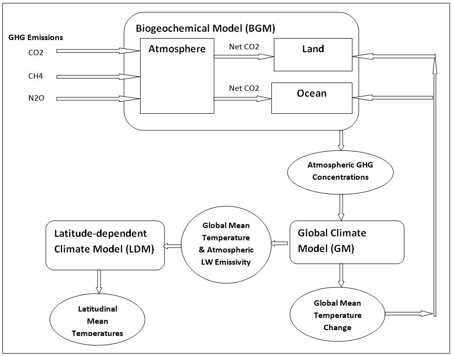
Atmospheric Greenhouse Gas (GHG) Concentrations
The atmospheric concentrations of GHGs are simulated in ClimateSim’s BGM module using a stock-and-flow model.
The simulation time period is from the year 2011 through the year 2100. The atmosphere starts with known concentrations of CO2, CH4 and N2O (10.3 PgC, 556 TgCH4 and 15.8 TgN respectively) in the year 2011. From there, new emissions enter the atmosphere each year based on the emissions trend of each GHG in the scenario being simulated and are accumulated in the atmosphere. Concurrently, some of the incremental CO2 emissions are removed each year by the land and ocean carbon uptake. Also, each year, some of the CH4 in the atmosphere reaches its average lifetime of 12.4 years and is removed from the atmosphere. (The average N2O lifetime exceeds a century and is currently not removed from the atmosphere in ClimateSim 1.0.)
ClimateSim uses a carbon uptake model with carbon and climate feedback (Friedlingstein 2006; Ciais 2013) to compute the total carbon uptake, ∆Cc, by land and ocean in each simulation year:
∆Cc= CL + βL ∆CO2 + γL ∆T + CO + βo ∆CO2 + γo ∆T
where
CL = Baseline Land Carbon Uptake, GtC/year
CO = Baseline Ocean Carbon Uptake, GtC/year
γL = Incremental Land Carbon Uptake (temp), GtC/K/year
γo = Incremental Ocean Carbon Uptake (temp), GtC/K/year
βL = Incremental Land Carbon Uptake (conc), GtC/ppm/year
βo = Incremental Ocean Carbon Uptake (conc), GtC/ppm/year
∆CO2 = Increase in atmospheric CO2 concentration in current year before uptake, ppm
∆T = Increase in temperature relative to baseline year
For carbon feedback, the model considers the incremental CO2 concentration from current-year emissions as a new perturbation and calculates the uptake fraction. For climate feedback, the model considers the total temperature increase from the baseline year (nominally 2011) to determine the impact on the total uptake. The model also caps the emissions reductions to 50% of the current-year emissions.
Global Response to GHG Perturbations
The global climate response to changes in atmospheric GHG perturbations is computed using a radiative forcing and climate sensitivity model in ClimateSim’s GM module.
Radiative forcing is calculated as follows (Box 2016; Ramaswamy 2001):
∆RFCO2 = 5.35 ln(C/C0)
where C = current CO2 concentration (ppm), C0 = pre-industrial concentration, ∆RF is in W/m2.
∆RFCH4 = 0.036 (M0.5 – M00.5 – f(M, N0) + f(M0, N0)
∆RFN2O = 0.036 (N0.5 – N00.5 – f(M0, N) + f(M0, N0)
f(M, N) = 0.47 ln(1 + 2.01e-5 (MN)0.75 + 5.32e-15 M (MN)1.52)
where M = CH4 concentration (ppb), N = N2O concentration (ppb), subscript 0 = pre-industrial concentrations.
Since the CH4 and N2O spectral overlaps are accounted for in the above equations, the three radiative forcings can be added to get a reasonable approximation of the total forcing at a global scale, ∆RF.
∆RF = ∆RFCO2 + ∆RFCH4 + ∆RFN2O
Next, a climate sensitivity factor λ is used to calculate a good indicator of the equilibrium global mean annual surface temperature change (in degrees K or C) relative to pre-industrial temperature:
∆T = λ ∆RF
λ has been shown to be a nearly invariant parameter in one-dimensional radiative-convective models, with a value of about 0.5 K/W/m2 (Ramaswamy 2001). λ captures the total climate feedback (including waver vapor, ice albedo, lapse rate and clouds) for a given total raw radiative forcing. In order to improve accuracy, we have used the total radiative forcings and GCM-based initial/final temperatures under four IPCC scenarios (RCP2.6, RCP4.5, RCP6.0, and RCP8.5 – see the Emissions Scenarios section below) to derive an empirical equation for λ, which yields sensitivity values in the range of 0.3 to 0.6 for most scenarios:
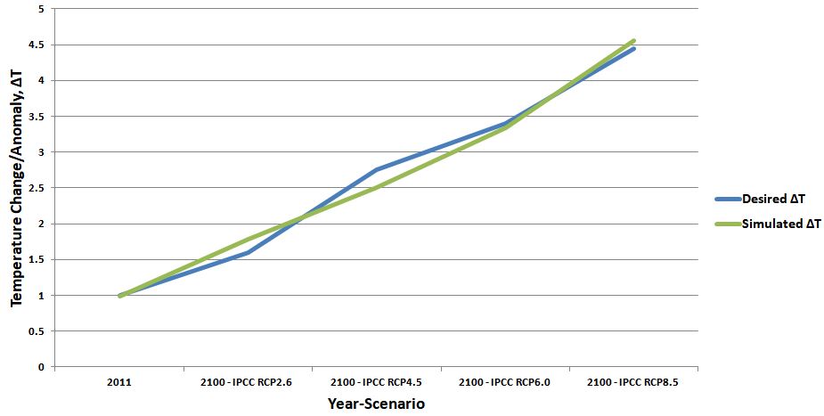
λ = 0.0092 (∆RF)2 - 0.1045 ∆RF + 0.5973
Using this sensitity factor, the chart below compares the ∆T from ClimateSim simulation to the desired values in the IPCC temperature ranges for the scenarios.
Given an absolute mean annual surface temperature Ts = Tb + ∆T, where Tb is the pre-industrial baseline temperature, we can estimate the atmospheric longwave emissivity or absorptivity at thermal equilibrium as
ε = 2 - 2 (1 – α - a/2) F/(σ Ts4)
where α = mean planetary albedo, a = atmospheric shortwave absorptivity, σ = Stefan-Boltzmann constant (W/m2/K4), F = mean solar flux at top of atmosphere (W/m2)
ε has been derived using the extended one-layer atmospheric model described in the next section. It represents a global, first-order estimate of the total impact of anthropogenic GHGs and other forcing agents (such as water vapor) in the atmosphere, and is used next in the latitude-dependent energy balance.
Latitude-dependent Response to GHG Perturbations
The latitudinal climate response to changes in atmospheric GHG perturbations is simulated based on energy-balance equations and an extended one-layer atmospheric model in ClimateSim’s LDM module.
The following set of equations represents the energy balance at the earth’s surface at latitude L (Box 2016):
x = sin(L)
F s(x) (1 – r(x)) – Flw(x) = 3.8 (T(x) – Ts)
where the first term on the left represents the incoming shortwave solar radiation at the surface, the second term on the left represents the outgoing net longwave radiation at the top of atmosphere, and the term on the right represents various transport losses including the equator-to-pole convective heat transport.
F = mean solar flux at top of atmosphere (W/m2)
T(x) = absolute mean annual temperature at latitude L
s(x) = normalized insolation factor to account for the latitudinal variation of solar radiation, at latitude L = 1 - 0.482 P2(x), where P2 is the Legendre polynomial of order 2.
r(x) = surface albedo, incorporating a simple ice-albedo model, at latitude L = 0.7 if T(x) < 230K; 0.1 if T(x) > 270K; (0.1 – 0.015) (T(x) – 270) otherwise
Flw(x) = net outgoing longwave radiation at latitude L = (1 - ε) σ T4(x) + e σ Ta4(x)
Ta(x) = absolute mean temperature of atmospheric layer at latitude L = ((a F + ε σ T4(x))/(2 ε σ))0.25
ClimateSim uses an iterative algorithm to converge on the latitudinal temperatures, T(x), in selected years.
Emissions Scenarios
The pre-defined emissions scenarios are listed in the table below. The four IPCC scenarios are based on AR5 (Edenhofer 2013) and the last four scenarios are based on mean/median trend data adapted from the Climate Action Tracker, with the CO2-equivalent emissions in each scenario mapped to CO2, CH4 and N2O as shown in the table. CH4 and N2O emissions are held constant at 2011 levels, and CO2 emissions vary in the 2012-2100 timeframe to match the total CO2-equivalent emissions.
| Emissions Scenario |
Mid-century Year |
In Mid-century Year |
In 2100 |
| CO2 |
CH4 |
N2O |
CO2 |
CH4 |
N2O |
| Negative Emissions |
2012 |
-10.00 |
0.00 |
0.00 |
-10.00 |
0.00 |
0.00 |
| Zero Emissions |
2012 |
0.00 |
0.00 |
0.00 |
0.00 |
0.00 |
0.00 |
| Default Emissions |
2050 |
14.90 |
827.10 |
22.60 |
9.80 |
554.30 |
15.10 |
| IPCC RCP2.6 |
2050 |
7.23 |
556.00 |
15.80 |
-0.29 |
556.00 |
15.80 |
| IPCC RCP4.5 |
2050 |
18.02 |
556.00 |
15.80 |
10.68 |
556.00 |
15.80 |
| IPCC RCP6.0 |
2050 |
24.01 |
556.00 |
15.80 |
23.37 |
556.00 |
15.80 |
| IPCC RCP8.5 |
2050 |
30.81 |
556.00 |
15.80 |
40.33 |
556.00 |
15.80 |
| Current Policy Projections (mean) |
2050 |
18.56 |
556.00 |
15.80 |
18.24 |
556.00 |
15.80 |
| Paris Pledges (mean) |
2030 |
14.17 |
556.00 |
15.80 |
8.55 |
556.00 |
15.80 |
| 2C Effort (median) |
2012 |
17.48 |
556.00 |
15.80 |
0.15 |
556.00 |
15.80 |
| 1.5C Effort (median) |
2012 |
17.48 |
556.00 |
15.80 |
-2.02 |
556.00 |
15.80 |
Units: CO2 emissions are in PgC; CH4 emissions are in TgCH4; N2O emissions are in TgN.
Key Model Parameters
GHG Parameters
CO2 Atmospheric Concentration Factor = 2.12 PgC/ppm
CH4 Atmospheric Concentration Factor = 2.7476 TgCH4/ppb
N2O Atmospheric Concentration Factor = 4.79 TgN/ppb
CO2 Preindustrial Atmospheric Concentration = 278 ppm
CH4 Preindustrial Atmospheric Concentration = 700 ppb
N2O Preindustrial Atmospheric Concentration = 270 ppb
CO2 Atmospheric Concentration in 2011 = 391 ppm
CH4 Atmospheric Concentration in 2011 = 1803 ppb
N2O Atmospheric Concentration in 2011 = 324 ppb
CO2 Emissions in 2011 = 10.3 PgC
CH4 Emissions in 2011 = 556 TgCH4
N2O Emissions in 2011 = 15.8 TgN
N2O 100-year Global Warming Potential = 28
CH4 100-year Global Warming Potential = 265
CH4 Mean Lifetime = 12.4 years
N2O Mean Lifetime = 121 years
Land/Ocean Carbon Uptake Parameters
Baseline Land Carbon Uptake, CL = 2.6 PgC/year
Baseline Ocean Carbon Uptake, CO = 2.3 PgC/year
Incremental Land Carbon Uptake (temp), γL = -79 GtC/K/year
Incremental Ocean Carbon Uptake (temp), γo = -30 GtC/K/year
Incremental Land Carbon Uptake (conc), βL = 1.35 GtC/ppm/year
Incremental Ocean Carbon Uptake (conc), βo = 1.13 GtC/ppm/year
Other Climate Parameters
Preindustrial Global Mean Surface Temperature (estimated) = 286.56 K
Mean Planetary Albedo, α = 0.3
Cloud Albedo = 0.5
Default Cloud Fraction = 0.5
Atmospheric SW Absorptivity, a = 0.15
Stefan-Boltzmann Constant, σ = 5.67e-8 W/m2/K4
Mean Solar Flux at Top of Atmosphere, F = F0/4 = 340.5 W/m2
We are planning several enhancements for ClimateSim 2.0, with a likely release date in late 2017. These enhancements include: multilayer atmosphere, latitude-dependent cloud fraction, and modeling geoengineering such as solar radiation management. We would love to hear your ideas on how we can make ClimateSim better and more useful as a fast and simple climate modeling/simulation tool as well as a science education tool. If you have suggestions or requests for specific enhancements, improvements or bug fixes – or any other feedback – please contact us at info@sciencebysimulation.com.
Box, M.A. and Box, G.P. 2016. Physics of Radiation and Climate. CRC Press, Boca Raton, FL.
Campbell, S.C. and Norman, J.M. 1998. An Introduction to Environmental Biophysics. Springer-Verlag, New York, NY.
Ciais, P., et al. 2013. Carbon and Other Biogeochemical Cycles. In: Climate Change 2013: The Physical Science Basis. Intergovernmental Panel on Climate Change.
Climate Action Tracker. 2017. Effect of Current Pledges and Policies on Global Temperature.
Edenhofer, O., et al. 2014. Technical Summary. In: Climate Change 2014: Mitigation of Climate Change. Intergovernmental Panel on Climate Change.
Friedlingstein, P., et al. 2006. Climate-Carbon Feedback Analysis: Results from the C4MIP Model Intercomparison. Journal of Climate, Vol. 19.
Fritz, S. 1949. The Albedo of Planet Earth and of Clouds. Journal of Meteorology, Vol. 6.
Forster, P., et al. 2007. Changes in Atmospheric Constituents and Radiative Forcing. In: Climate Change 2007: The Physical Science Basis. Intergovernmental Panel on Climate Change.
Hawkins, E., et al. 2017. Estimating Changes in Global Temperature since the Pre-industrial Period. Bulletin of the American Meteorological Society, Vol. 98.
Myhre, G., et al. 2013. Anthropogenic and Natural Radiative Forcing. In: Climate Change 2013: The Physical Science Basis. Intergovernmental Panel on Climate Change.
Ramaswamy, V., et al. 2001. Radiative Forcing of Climate Change. In: Climate Change 2001: The Scientific Basis. Intergovernmental Panel on Climate Change.